Faster RCNN代码解析
本文最后更新于:2021年1月8日 晚上
本文转载自GiantPandaCV,感谢整理分享。
📖 Faster RCNN整体结构
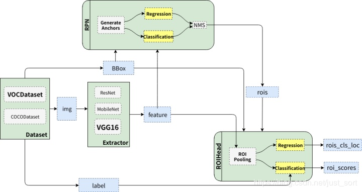
Faster RCNN大概可以分成绿色描述的个部分,即:
DataSet:代表数据集,典型的比如VOC和COCO。Extrator:特征提取器,也即是我们常说的Backbone网络,典型的有VGG和ResNet。RPN:全称Region Proposal Network,负责产生候选区域(rois),每张图大概给出2000个候选框。RoIHead:负责对rois进行分类和回归微调。
所以Faster RCNN的流程可以总结为:
原始图像—->特征提取———>RPN产生候选框———>对候选框进行分类和回归微调。
🔎 Faster RCNN的四个模块
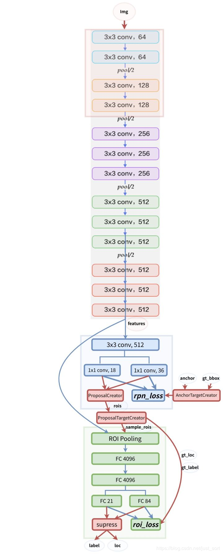
Faster R-CNN是目标检测中较早提出来的两阶段网络,其网络架构如下图所示:
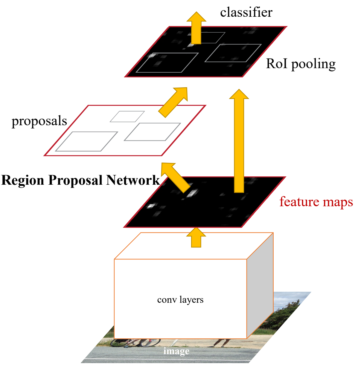
可以看出可以大体分为四个部分:
Conv Layers卷积神经网络用于提取特征,得到feature map。RPN网络,用于提取Region of Interests(RoI)。RoI pooling, 用于综合RoI和feature map, 得到固定大小的resize后的feature。classifier, 用于分类RoI属于哪个类别。
1. Conv Layers
在Conv Layers中,对输入的图片进行卷积和池化,用于提取图片特征,最终希望得到的是feature map。在Faster R-CNN中,先将图片Resize到固定尺寸,然后使用了VGG16中的13个卷积层、13个ReLU层、4个manpooling层。(VGG16中进行了5次下采样,这里舍弃了第四次下采样后的部分,将剩下部分作为Conv Layer提取特征。)
与YOLOv3不同,Faster R-CNN下采样后的分辨率为原始图片分辨率的1/16(YOLOv3是变为原来的1/32)。feature map的分辨率要比YOLOv3的Backbone得到的分辨率要大,这也可以解释为何Faster R-CNN在小目标上的检测效果要优于YOLOv3。
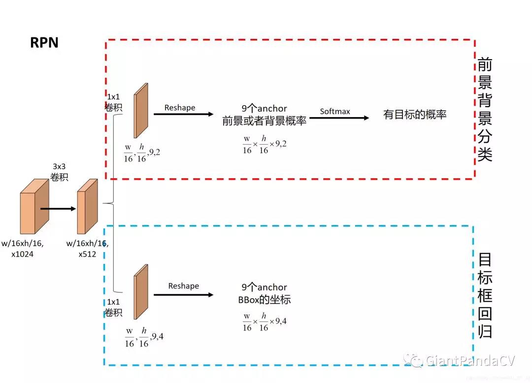
2. Region Proposal Network
简称RPN网络,用于推荐候选区域(Region of Interests),接受的输入为原图片经过Conv Layer后得到的feature map。
上图参考的实现是:https://github.com/ruotianluo/pytorch-faster-rcnn
RPN网络将feature map作为输入,然后用了一个3x3卷积将filter减半为512,然后进入两个分支:
一个分支用于计算对应anchor的foreground和background的概率,目标是foreground。
一个分支用于计算对应anchor的Bounding box的偏移量,来获得其目标的定位。
通过RPN网络,我们就得到了每个anchor是否含有目标和在含有目标情况下目标的位置信息。
对比RPN和YOLOv3:
RPN: 分两个分支,一个分支预测目标框,一个分支预测前景或者背景。将两个工作分开来做的,并且其中前景背景预测分支功能是判断这个anchor是否含有目标,并不会对目标进行分类。另外就是anchor的设置是通过先验得到的。
YOLOv3: 将整个问题当做回归问题,直接就可以获取目标类别和坐标。Anchor是通过IoU聚类得到的。
区别:Anchor的设置,Ground truth和Anchor的匹配细节不一样。
联系:两个都是在最后的feature map(w/16,h/16或者w/32,h/32)上每个点都分配了多个anchor,然后进行匹配。虽然具体实现有较大的差距,但是这个想法有共同点。
3. ROI Pooling
这里看一个来自deepsense.ai提供的例子:
RoI Pooling输入是feature map和RoIs:
假设feature map是如下内容:
RPN提供的其中一个RoI为:左上角坐标(0,3),右下角坐标(7,8)
然后将RoI对应到feature map上的部分切割为2x2大小的块:
将每个块做类似max pooling的操作,得到以下结果:
以上就是ROI pooling的完整操作,想一想为何要这样做?
- 保证无论输入特征图尺寸如何,输入到后续全连接层的特征图尺寸固定,避免因图像裁剪等造成像素缺失。
- 输入特征图尺寸为M×N,ROI池化层先将其映射为M/16×N/16,结合ROI获得原始特征图的区域建议坐标,然后将该区域分块,分别进行max pooling,得到最终的区域建议
在RPN阶段,我们得知了当前图片是否有目标,在有目标情况下目标的位置。现在唯一缺少的信息就是这个目标到底属于哪个类别(通过RPN只能得知这个目标属于前景,但并不能得到具体类别)。
如果想要得知这个目标属于哪个类别,最简单的想法就是将得到的框内的图片放入一个CNN进行分类,得到最终类别。这就涉及到最后一个模块:classification
4. Classification
ROI Pooling后得到的是大小一致的feature map,然后分为两个分支,靠下的一个分支去进行分类,上一个分支是用于Bounding box回归。如下图所示(来自知乎):
分类这个分支很容易理解,用于计算到底属于哪个类别。Bounding box回归的分支用于调整RPN预测得到的Bounding box,让回归的结果更加精确。
⛳ 数据预处理及实现细节
首先让我们进入到这个Pytorch的Faster RCNN工程:https://github.com/chenyuntc/simple-faster-rcnn-pytorch。数据预处理的相关细节都在data这个文件夹下面,实现流程图如下:

data/dataset.py
# 去正则化,img维度为[[B,G,R],H,W],因为caffe预训练模型输入为BGR 0-255图片,pytorch预训练模型采用RGB 0-1图片
def inverse_normalize(img):
    if opt.caffe_pretrain:
        # [122.7717, 115.9465, 102.9801]reshape为[3,1,1]与img维度相同就可以相加了,
        # pytorch_normalize之前有减均值预处理,现在还原回去。
        img = img + (np.array([122.7717, 115.9465, 102.9801]).reshape(3, 1, 1))
        # 将BGR转换为RGB图片(python [::-1]为逆序输出)
        return img[::-1, :, :]
    # pytorch_normalze中标准化为 减均值除以标准差,现在乘以标准差加上均值还原回去,转换为0-255
    return (img * 0.225 + 0.45).clip(min=0, max=1) * 255

# 采用pytorch预训练模型对图片预处理(归一化),函数输入的img为 0~1
# 函数输出为 -1~1,RGB,减去均值再除以标准差
def pytorch_normalze(img):
    """
    https://github.com/pytorch/vision/issues/223
    return appr -1~1 RGB
    """
    # #transforms.Normalize使用如下公式进行归一化
    # channel=(channel-mean)/std,转换为[-1,1]
    normalize = tvtsf.Normalize(mean=[0.485, 0.456, 0.406],
                                std=[0.229, 0.224, 0.225])
    # nddarry->Tensor
    img = normalize(t.from_numpy(img))
    return img.numpy()

# 采用caffe预训练模型时对输入图像进行标准化,函数输入的img为 0~1
# 函数输出为 -125~125,BGR,只减了均值,未除标准差
def caffe_normalize(img):
    """
    return appr -125-125 BGR
    """
    # RGB-BGR
    img = img[[2, 1, 0], :, :]  # RGB-BGR
    img = img * 255
    # 转换为与img维度相同
    mean = np.array([122.7717, 115.9465, 102.9801]).reshape(3, 1, 1)
    # 减均值操作
    img = (img - mean).astype(np.float32, copy=True)
    return img

# 函数输入的img为0-255
def preprocess(img, min_size=600, max_size=1000):
    # 图片进行缩放,使得长边小于等于1000,短边小于等于600(至少有一个等于)。
    # 对相应的bounding boxes 也也进行同等尺度的缩放。
    C, H, W = img.shape
    scale1 = min_size / min(H, W)
    scale2 = max_size / max(H, W)
    # 选小的比例,这样长和宽都能放缩到规定的尺寸
    scale = min(scale1, scale2)
    img = img / 255.
    # resize到(H * scale, W * scale)大小,anti_aliasing为是否采用高斯滤波
    img = sktsf.resize(img, (C, H * scale, W * scale), mode='reflect',anti_aliasing=False)
    #调用pytorch_normalze或者caffe_normalze对图像进行正则化,输入为0~1
    if opt.caffe_pretrain:
        normalize = caffe_normalize
    else:
        normalize = pytorch_normalze
    return normalize(img)

# 对原图和bbox进行缩放、随机翻转
class Transform(object):

    def __init__(self, min_size=600, max_size=1000):
        self.min_size = min_size
        self.max_size = max_size

    def __call__(self, in_data):
        img, bbox, label = in_data
        _, H, W = img.shape
        # 调用前面定义的preprocess函数进行图像等比例缩放
        img = preprocess(img, self.min_size, self.max_size)
        _, o_H, o_W = img.shape
        # 得出缩放比因子
        scale = o_H / H
        # bbox按照与原图等比例缩放
        bbox = util.resize_bbox(bbox, (H, W), (o_H, o_W))

        # 将图片进行随机水平翻转,没有进行垂直翻转
        img, params = util.random_flip(
            img, x_random=True, return_param=True)
        # 同样地将bbox进行与对应图片同样的水平翻转
        bbox = util.flip_bbox(
            bbox, (o_H, o_W), x_flip=params['x_flip'])

        return img, bbox, label, scale

# 训练集样本的生成
class Dataset:
    def __init__(self, opt):
        self.opt = opt
         # 实例化 VOCBboxDataset 类
        self.db = VOCBboxDataset(opt.voc_data_dir)
        # 实例化 Transform 类
        self.tsf = Transform(opt.min_size, opt.max_size)

    # __ xxx__运行Dataset类时自动运行

    def __getitem__(self, idx):
        # 调用VOCBboxDataset中的get_example()从数据集存储路径中将img, bbox, label, difficult 一个个的获取出来
        ori_img, bbox, label, difficult = self.db.get_example(idx)
        # 调用前面的Transform函数将图片,label进行最小值最大值放缩归一化,
        # 重新调整bboxes的大小,然后随机反转,最后将数据集返回
        img, bbox, label, scale = self.tsf((ori_img, bbox, label))
        # TODO: check whose stride is negative to fix this instead copy all
        # some of the strides of a given numpy array are negative.
        return img.copy(), bbox.copy(), label.copy(), scale

    def __len__(self):
        return len(self.db)

# 测试集样本的生成
class TestDataset:
    def __init__(self, opt, split='test', use_difficult=True):
        self.opt = opt
        # 此处设置了use_difficult,
        self.db = VOCBboxDataset(opt.voc_data_dir, split=split, use_difficult=use_difficult)

    def __getitem__(self, idx):
        ori_img, bbox, label, difficult = self.db.get_example(idx)
        # 对原图进行缩放
        img = preprocess(ori_img)
        return img, ori_img.shape[1:], bbox, label, difficult

    def __len__(self):
        return len(self.db)
data/voc_dataset.py
class VOCBboxDataset:

    def __init__(self, data_dir, split='trainval',
                 use_difficult=False, return_difficult=False,
                 ):

        # if split not in ['train', 'trainval', 'val']:
        #     if not (split == 'test' and year == '2007'):
        #         warnings.warn(
        #             'please pick split from \'train\', \'trainval\', \'val\''
        #             'for 2012 dataset. For 2007 dataset, you can pick \'test\''
        #             ' in addition to the above mentioned splits.'
        #         )

        # id_list_file为split.txt,split为'trainval'或者'test'
        id_list_file = os.path.join(data_dir, 'ImageSets/Main/{0}.txt'.format(split))
        # id_为每个样本文件名
        self.ids = [id_.strip() for id_ in open(id_list_file)]  # strip()会去掉前后空格
        # 写到/VOC2007/的路径
        self.data_dir = data_dir
        self.use_difficult = use_difficult
        self.return_difficult = return_difficult
        # 20类
        self.label_names = VOC_BBOX_LABEL_NAMES

    # trainval.txt有5011个,test.txt有210个
    def __len__(self):
        return len(self.ids)

    def get_example(self, i):
        #读入xml标签文件
        id_ = self.ids[i]
        # ElementTree 调用parse()方法,返回解析树
        anno = ET.parse(os.path.join(self.data_dir, 'Annotations', id_ + '.xml'))
        bbox = list()
        label = list()
        difficult = list()
        #解析xml文件
        for obj in anno.findall('object'):
            # 标为difficult的目标在测试评估中一般会被忽略
            if not self.use_difficult and int(obj.find('difficult').text) == 1:
                continue
            #xml文件中包含object name和difficult(0或者1,0代表容易检测)
            difficult.append(int(obj.find('difficult').text))
            # bndbox(xmin,ymin,xmax,ymax),表示框左下角和右上角坐标
            bndbox_anno = obj.find('bndbox')
            # 让坐标基于(0,0),意义何在?
            bbox.append([
                int(bndbox_anno.find(tag).text) - 1
                for tag in ('ymin', 'xmin', 'ymax', 'xmax')])
            # 框中object name
            name = obj.find('name').text.lower().strip()
            label.append(VOC_BBOX_LABEL_NAMES.index(name))
        # 所有object的bbox坐标存在列表里
        bbox = np.stack(bbox).astype(np.float32)
        # 所有object的label存在列表里
        label = np.stack(label).astype(np.int32)
        # PyTorch 不支持 np.bool,所以这里转换为uint8
        difficult = np.array(difficult, dtype=np.bool).astype(np.uint8)

        # 根据图片编号在/JPEGImages/取图片
        img_file = os.path.join(self.data_dir, 'JPEGImages', id_ + '.jpg')
        # 如果color=True,则转换为RGB图
        img = read_image(img_file, color=True)

        # if self.return_difficult:
        #     return img, bbox, label, difficult
        return img, bbox, label, difficult

    # 一般如果想使用索引访问元素时,就可以在类中定义这个方法(__getitem__(self, key) )
    __getitem__ = get_example

# 类别和名字对应的列表
VOC_BBOX_LABEL_NAMES = (
    'aeroplane',
    'bicycle',
    'bird',
    'boat',
    'bottle',
    'bus',
    'car',
    'cat',
    'chair',
    'cow',
    'diningtable',
    'dog',
    'horse',
    'motorbike',
    'person',
    'pottedplant',
    'sheep',
    'sofa',
    'train',
'tvmonitor')再接下来是utils.py里面一些用到的相关函数的注释,只选了其中几个,并且有一些函数没有用到,全部放上来篇幅太多:
def resize_bbox(bbox, in_size, out_size):
    # 根据图片resize的情况来缩放bbox
    bbox = bbox.copy()
    #  #获得与原图同样的缩放比
    y_scale = float(out_size[0]) / in_size[0]
    x_scale = float(out_size[1]) / in_size[1]
    # #按与原图同等比例缩放bbox
    bbox[:, 0] = y_scale * bbox[:, 0]
    bbox[:, 2] = y_scale * bbox[:, 2]
    bbox[:, 1] = x_scale * bbox[:, 1]
    bbox[:, 3] = x_scale * bbox[:, 3]
    return bbox


def flip_bbox(bbox, size, y_flip=False, x_flip=False):
    # 根据图片flip的情况来flip bbox
    H, W = size #缩放后图片的size
    bbox = bbox.copy()
    if y_flip:  #进行垂直翻转
        # bbox为(channel,(ymin,xmin,ymax,xmax))
        y_max = H - bbox[:, 0]
        y_min = H - bbox[:, 2]
        bbox[:, 0] = y_min
        bbox[:, 2] = y_max
    if x_flip: #进行水平翻转
        x_max = W - bbox[:, 1]
        x_min = W - bbox[:, 3] #计算水平翻转后左下角和右上角的坐标
        bbox[:, 1] = x_min
        bbox[:, 3] = x_max
    return bbox

def random_flip(img, y_random=False, x_random=False,
                return_param=False, copy=False):
    # 数据增强,随机翻转
    y_flip, x_flip = False, False
    # 随机选择图片是否进行垂直、水平翻转
    if y_random:
        y_flip = random.choice([True, False])
    if x_random:
        x_flip = random.choice([True, False])

    if y_flip:
        # channel,height,weight
        img = img[:, ::-1, :]
    if x_flip:
        # python [::-1]为逆序输出,这里指水平翻转
        img = img[:, :, ::-1]

    if copy:
        img = img.copy()

    if return_param:
        #返回img和x_flip(为了让bbox有同样的水平翻转操作)
        return img, {'y_flip': y_flip, 'x_flip': x_flip}
    else:
        return img
🎫 RPN和ROI Head
原始图片首先会经过一个特征提取器Extrator(这里是VGG16),在原始论文中作者使用了Caffe的预训练模型。同时将VGG16模型的前4层卷积层的参数冻结(在Caffe中将其学习率设为0),并将最后3层全连接层的前两层保留并用来初始化ROI Head里面部分参数。我们可以将Extrator用下图来表示:

可以看到对于一个尺寸为H×W×C的图片,经过这个特征提取网络之后会得到一个H/16 × W/16 × 512的特征图,也即是图中的红色箭头代表的Features。
从整体结构图中,我们可以看到RPN这个候选框生成网络接收了两个输入,一个是特征图也就是我们刚提到的,另外一个是数据集提供的GT Box,这里面究竟是怎么操作呢?
Anchor生成
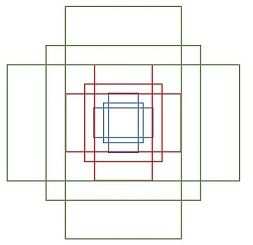
我们知道RPN网络使用来提取候选框的,它最大的贡献就在于它提出了一个Anchor的思想,这也是后面One-Stage以及Two-Stage的各类目标检测算法的出发点,Anchor表示的是大小和尺寸固定的候选框,论文中用到了三种比例和三种尺寸,也就是说对于特征图的每个点都将产生9种不同大小的Anchor候选框,其中三种尺寸分别是128、256、512,而三种比例分别为:1:2、2:1、1:1。Faster RCNN的九种Anchor的示意图如下:
这里我们先来看一下生成Anchor的过程,具体是在model/util文件夹下。我们首先来看bbox_tools.py文件,其中涉及到了RCNN中提到的边框回归公式,$\hat{G}$代表候选框,而回归学习就是学习 $d{x},d{y}, d{h},d{w}$ 这 4 个偏移量 。
真正的目标框G和候选框P之间的偏移可以表示为:
def loc2bbox(src_bbox, loc):
    # 已知源边界框src_bbox和位置偏差loc,求目标框dst_bbox
    # src_bbox:shape为(R,4),R为bbox个数,4为左上角和右下角四个坐标
    # scr_bbox=[[ymin,xmin,ymax,xmax]
    # 			[ymin,xmin,ymax,xmax]
    #           ...
    #			[ymin,xmin,ymax,xmax]]
    #
    # loc为[[dy,dx,dh,dw,dy,dx,dh,dw...]  # 图片1的边界框位置偏差?
    #      [dy,dx,dh,dw,dy,dx,dh,dw...]
    #      ...
    #      [dy,dx,dh,dw,dy,dx,dh,dw...]]

    if src_bbox.shape[0] == 0:
        return np.zeros((0, 4), dtype=loc.dtype)

    src_bbox = src_bbox.astype(src_bbox.dtype, copy=False)

    # src_height为Ph,src_width为Pw,src_ctr_y为Py,src_ctr_x为Px
    src_height = src_bbox[:, 2] - src_bbox[:, 0]  # ymax-ymin
    src_width = src_bbox[:, 3] - src_bbox[:, 1]   # xmax-xmin
    src_ctr_y = src_bbox[:, 0] + 0.5 * src_height # y_min+0.5h,计算出中心点坐标
    src_ctr_x = src_bbox[:, 1] + 0.5 * src_width  # x_min+0.5w

    # python [start:stop:step]
    dy = loc[:, 0::4]
    dx = loc[:, 1::4]
    dh = loc[:, 2::4]
    dw = loc[:, 3::4]

    # RCNN中提出的边框回归:寻找原始proposal与近似目标框G之间的映射关系,公式在上面
    # 得到回归后的目标框的高度、宽度和中心点坐标(Gx,Gy,Gh,Gw)
    ctr_y = dy * src_height[:, np.newaxis] + src_ctr_y[:, np.newaxis] # ctr_y为Gy
    ctr_x = dx * src_width[:, np.newaxis] + src_ctr_x[:, np.newaxis] # ctr_x为Gx
    h = np.enp(dh) * src_height[:, np.newaxis] # h为Gh
    w = np.enp(dw) * src_width[:, np.newaxis] # w为Gw


    # 由中心点转换为左上角和右下角坐标
    dst_bbox = np.zeros(loc.shape, dtype=loc.dtype)
    dst_bbox[:, 0::4] = ctr_y - 0.5 * h  # y_min
    dst_bbox[:, 1::4] = ctr_x - 0.5 * w  # x_min
    dst_bbox[:, 2::4] = ctr_y + 0.5 * h  # y_max
    dst_bbox[:, 3::4] = ctr_x + 0.5 * w  # x_max

    return dst_bbox


# 已知源框src_bbox和目标框dst_bbox,求出其位置偏差
def bbox2loc(src_bbox, dst_bbox):

    # 计算出源框中心点坐标
    height = src_bbox[:, 2] - src_bbox[:, 0] # y_max-y_min
    width = src_bbox[:, 3] - src_bbox[:, 1] # x_max-x_min
    ctr_y = src_bbox[:, 0] + 0.5 * height
    ctr_x = src_bbox[:, 1] + 0.5 * width

    # 计算出目标框中心点坐标
    base_height = dst_bbox[:, 2] - dst_bbox[:, 0]
    base_width = dst_bbox[:, 3] - dst_bbox[:, 1]
    base_ctr_y = dst_bbox[:, 0] + 0.5 * base_height
    base_ctr_x = dst_bbox[:, 1] + 0.5 * base_width

    # 求出最小的正数
    eps = np.finfo(height.dtype).eps
    # 将height,width与其比较保证全部是非负
    height = np.maximum(height, eps)
    width = np.maximum(width, eps)

    # 根据上面的公式二计算dx,dy,dh,dw
    dy = (base_ctr_y - ctr_y) / height
    dx = (base_ctr_x - ctr_x) / width
    dh = np.log(base_height / height)
    dw = np.log(base_width / width)

    # np.vstack按照行的顺序把数组给堆叠起来
    loc = np.vstack((dy, dx, dh, dw)).transpose()
    return loc


# 求两个bbox的相交的交并比
def bbox_iou(bbox_a, bbox_b):
    # bbox_a=[[ymin,xmin,ymax,xmax]
    # 		  [ymin,xmin,ymax,xmax]
    #         ...
    #		  [ymin,xmin,ymax,xmax]]

    # 确保bbox第二维为bbox的四个坐标(ymin,xmin,ymax,xmax)
    if bbox_a.shape[1] != 4 or bbox_b.shape[1] != 4:
        raise IndexError

    # top left
    # l为交叉部分框左上角坐标最大值,为了利用numpy的广播性质,
    # bbox_a[:, None, :2]的shape是(N,1,2),bbox_b[:, :2]的shape是(K,2)
    # 由numpy的广播性质,两个数组shape都变成(N,K,2),也就是对a里每个bbox都分别和b里的每个bbox求左上角点坐标最大值
    tl = np.maximum(bbox_a[:, None, :2], bbox_b[:, :2])

    # bottom right
    # br为交叉部分框右下角坐标最小值
    br = np.minimum(bbox_a[:, None, 2:], bbox_b[:, 2:])

    # 所有坐标轴上tl<br时,返回数组元素的乘积(y1max-yimin)X(x1max-x1min),
    # bboxa与bboxb相交区域的面积
    area_i = np.prod(br - tl, axis=2) * (tl < br).all(axis=2)
    # 计算bboxa的面积
    area_a = np.prod(bbox_a[:, 2:] - bbox_a[:, :2], axis=1)
    # 计算bboxb的面积
    area_b = np.prod(bbox_b[:, 2:] - bbox_b[:, :2], axis=1)
    # 计算IOU
    return area_i / (area_a[:, None] + area_b - area_i)


def __test():
    pass


if __name__ == '__main__':
    __test()


# 对特征图features以基准长度为16、选择合适的ratios和scales取基准锚点
 # anchor_base。(选择长度为16的原因是图片大小为600*800左右,基准长度
 # 16对应的原图区域是256*256,考虑放缩后的大小有128*128,512*512比较合适)
def generate_anchor_base(base_size=16, ratios=[0.5, 1, 2],
                         anchor_scales=[8, 16, 32]):
    # 根据基准点生成9个基本的anchor的功能,ratios=[0.5,1,2],anchor_scales=
    # [8,16,32]是长宽比和缩放比例,anchor_scales也就是在base_size的基础上再增
    # 加的量,本代码中对应着三种面积的大小(16*8)^2 ,(16*16)^2  (16*32)^2
    # 也就是128,256,512的平方大小

    py = base_size / 2.
    px = base_size / 2.

    #(9,4),注意:这里只是以特征图的左上角点为基准产生的9个anchor,
    anchor_base = np.zeros((len(ratios) * len(anchor_scales), 4),
                           dtype=np.float32)
    # six.moves 是用来处理那些在python2 和 3里面函数的位置有变化的,
    # 直接用six.moves就可以屏蔽掉这些变化
    for i in six.moves.range(len(ratios)):
        for j in six.moves.range(len(anchor_scales)):
            # 生成9种不同比例的h和w
            h = base_size * anchor_scales[j] * np.sqrt(ratios[i])
            w = base_size * anchor_scales[j] * np.sqrt(1. / ratios[i])

            index = i * len(anchor_scales) + j
            # 计算出anchor_base画的9个框的左下角和右上角的4个anchor坐标值
            anchor_base[index, 0] = py - h / 2.
            anchor_base[index, 1] = px - w / 2.
            anchor_base[index, 2] = py + h / 2.
            anchor_base[index, 3] = px + w / 2.
return anchor_base在上面的generate_anchor_base函数中,输出Anchor的形状以及这9个Anchor的左上右下坐标如下:
# 这9个anchor形状为:
90.50967 *181.01933    = 128^2
181.01933 * 362.03867 = 256^2
362.03867 * 724.07733 = 512^2
128.0 * 128.0 = 128^2
256.0 * 256.0 = 256^2
512.0 * 512.0 = 512^2
181.01933 * 90.50967   = 128^2
362.03867 * 181.01933 = 256^2
724.07733 * 362.03867 = 512^2

# 9个anchor的左上右下坐标:
-37.2548 -82.5097 53.2548 98.5097
-82.5097 -173.019 98.5097 189.019
-173.019 -354.039 189.019 370.039
-56 -56 72 72
-120 -120 136 136
-248 -248 264 264
-82.5097 -37.2548 98.5097 53.2548
-173.019 -82.5097 189.019 98.5097
-354.039 -173.019 370.039 189.019
需要注意的是:
anchor_base = np.zeros((len(ratios) * len(anchor_scales), 4), dtype=np.float32)这行代码表示的是只是以特征图的左上角为基准产生的9个Anchor,而我们知道Faster RCNN是会在特征图的每个点产生9个Anchor的,这个过程在什么地方呢?答案是在mode/region_proposal_network.py里面,这里面的_enumerate_shifted_anchor这个函数就实现了这一功能,接下来我们就仔细看看这个函数是如何产生整个特征图的所有Anchor的(一共20000+个左右Anchor,另外产生的Anchor坐标会截断到图像坐标范围里面)。下面来看看model/region_proposal_network.py里面的_enumerate_shifted_anchor函数
# 利用anchor_base生成所有对应feature map的anchor
def _enumerate_shifted_anchor(anchor_base, feat_stride, height, width):
    # Enumerate all shifted anchors:
    #
    # add A anchors (1, A, 4) to
    # cell K shifts (K, 1, 4) to get
    # shift anchors (K, A, 4)
    # reshape to (K*A, 4) shifted anchors
    # return (K*A, 4)

    # !TODO: add support for torch.CudaTensor
    # np = cuda.get_array_module(anchor_base)
    # it seems that it can't be boosed using GPU
    import numpy as np
    # 纵向偏移量(0,16,32,...)
    shift_y = np.arange(0, height * feat_stride, feat_stride)
    # 横向偏移量(0,16,32,...)
    shift_x = np.arange(0, width * feat_stride, feat_stride)
    # shift_x = [[0,16,32,..],[0,16,32,..],[0,16,32,..]...],
    # shift_y = [[0,0,0,..],[16,16,16,..],[32,32,32,..]...],
    # 就是形成了一个纵横向偏移量的矩阵,也就是特征图的每一点都能够通过这个
    # 矩阵找到映射在原图中的具体位置!
    shift_x, shift_y = np.meshgrid(shift_x, shift_y)
    # #经过刚才的变化,其实大X,Y的元素个数已经相同,看矩阵的结构也能看出,
    # 矩阵大小是相同的,X.ravel()之后变成一行,此时shift_x,shift_y的元
    # 素个数是相同的,都等于特征图的长宽的乘积(像素点个数),不同的是此时
    # 的shift_x里面装得是横向看的x的一行一行的偏移坐标,而此时的y里面装
    # 的是对应的纵向的偏移坐标!下图显示 np.meshgrid(),shift_y.ravel()
    # 操作示例
    shift = np.stack((shift_y.ravel(), shift_x.ravel(),
                      shift_y.ravel(), shift_x.ravel()), axis=1)
    # A=9
    A = anchor_base.shape[0]
    # 读取特征图中元素的总个数
    K = shift.shape[0]
    #用基础的9个anchor的坐标分别和偏移量相加,最后得出了所有的anchor的坐标,
    # 四列可以堪称是左上角的坐标和右下角的坐标加偏移量的同步执行,飞速的从
    # 上往下捋一遍,所有的anchor就都出来了!一共K个特征点,每一个有A(9)个
    # 基本的anchor,所以最后reshape((K*A),4)的形式,也就得到了最后的所有
    # 的anchor左下角和右上角坐标.
    anchor = anchor.reshape((K * A, 4)).astype(np.float32)

    anchor = anchor_base.reshape((1, A, 4)) + \
             shift.reshape((1, K, 4)).transpose((1, 0, 2))
    anchor = anchor.reshape((K * A, 4)).astype(np.float32)
return anchor我们结合一个例子来看一下shift_x, shift_y = np.meshgrid(shift_x, shift_y)函数操这个函数到底执行了什么操作?其中np就是numpy。
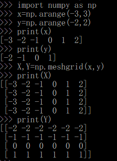
然后shift = np.stack((shift_y.ravel(), shift_x.ravel(),shift_y.ravel(), shift_x.ravel()), axis=1)这行代码则是产生坐标偏移对,一个是x方向,一个是y方向。
另外一个问题是这里为什么需要将特征图对应回原图呢?这是因为我们要框住的目标是在原图上,而我们选Anchor是在特征图上,Pooling之后特征之间的相对位置不变,但是尺寸已经减少为了原始图的$1/16$,而我们的Anchor是为了框住原图上的目标而非特征图上的,所以注意一下Anchor一定指的是针对原图的,而非特征图。
接下来我们看看训练RPN的一些细节,RPN的总体架构如下图所示:
首先我们要明确Anchor的数量是和特征图相关的,不同的特征图对应的Anchor数量也不一样。RPN在Extractor输出的特征图基础上先增加了一个$3×3$卷积,然后利用两个$1×1$卷积分别进行二分类和位置回归。进行分类的卷积核通道数为$9×2$(9个Anchor,每个Anchor 二分类,使用交叉熵损失),进行回归的卷积核通道数为$9×4$(9个Anchor,每个Anchor有4个位置参数)。RPN是一个全卷积网络,这样对输入图片的尺寸是没有要求的。
接下来我们就要讲到今天的重点部分了,即AnchorTargetCreator,ProposalCreator,ProposalTargetCreator,也就是ROI Head最核心的部分:
AnchorTargetCreator
AnchorTargetCreator就是将20000多个候选的Anchor选出256个Anchor进行分类和回归,选择过程如下:
- 对于每一个GT bbox,选择和它交并比最大的一个Anchor作为正样本。
- 对于剩下的Anchor,从中选择和任意一个GT bbox交并比超过0.7的Anchor作为正样本,正样本数目不超过128个。
- 随机选择和GT bbox交并比小于0.3的Anchor作为负样本,负样本和正样本的总数为256。
对于每一个Anchor来说,GT_Label要么为1(前景),要么为0(背景),而GT_Loc则是由4个位置参数组成,也就是上面讲的目标框和候选框之间的偏移。
计算分类损失使用的是交叉熵损失,而计算回归损失则使用了SmoothL1Loss,在计算回归损失的时候只计算正样本(前景)的损失,不计算负样本的损失。
代码实现在model/utils/creator_tool.py里面,具体如下:
# AnchorTargetCreator作用是生成训练要用的anchor(正负样本
# 各128个框的坐标和256个label(0或者1))
# 利用每张图中bbox的真实标签来为所有任务分配ground truth
class AnchorTargetCreator(object):


    def __init__(self,
                 n_sample=256,
                 pos_iou_thresh=0.7, neg_iou_thresh=0.3,
                 pos_ratio=0.5):
        self.n_sample = n_sample
        self.pos_iou_thresh = pos_iou_thresh
        self.neg_iou_thresh = neg_iou_thresh
        self.pos_ratio = pos_ratio

    def __call__(self, bbox, anchor, img_size):
        # 特征图大小
        img_H, img_W = img_size
        # 一般对应20000个左右anchor
        n_anchor = len(anchor)
        # 将那些超出图片范围的anchor全部去掉,只保留位于图片内部的序号
        inside_index = _get_inside_index(anchor, img_H, img_W)
        # 保留位于图片内部的anchor
        anchor = anchor[inside_index]
        # 筛选出符合条件的正例128个负例128并给它们附上相应的label
        argmax_ious, label = self._create_label(
            inside_index, anchor, bbox)

        # 计算每一个anchor与对应bbox求得iou最大的bbox计算偏移
        # 量(注意这里是位于图片内部的每一个)
        loc = bbox2loc(anchor, bbox[argmax_ious])

        # 将位于图片内部的框的label对应到所有生成的20000个框中
        # (label原本为所有在图片中的框的)
        label = _unmap(label, n_anchor, inside_index, fill=-1)
        # 将回归的框对应到所有生成的20000个框中(label原本为
        # 所有在图片中的框的)
        loc = _unmap(loc, n_anchor, inside_index, fill=0)

        return loc, label
    # 下面为调用的_creat_label() 函数
    def _create_label(self, inside_index, anchor, bbox):
        # inside_index为所有在图片范围内的anchor序号
        label = np.empty((len(inside_index),), dtype=np.int32)
        # #全部填充-1
        label.fill(-1)
        # 调用_calc_ious()函数得到每个anchor与哪个bbox的iou最大
        # 以及这个iou值、每个bbox与哪个anchor的iou最大(需要体会从
        # 行和列取最大值的区别)
        argmax_ious, max_ious, gt_argmax_ious = \
            self._calc_ious(anchor, bbox, inside_index)

        # #把每个anchor与对应的框求得的iou值与负样本阈值比较,若小
        # 于负样本阈值,则label设为0,pos_iou_thresh=0.7,
        # neg_iou_thresh=0.3
        label[max_ious < self.neg_iou_thresh] = 0

        # 把与每个bbox求得iou值最大的anchor的label设为1
        label[gt_argmax_ious] = 1

        # 把每个anchor与对应的框求得的iou值与正样本阈值比较,
        # 若大于正样本阈值,则label设为1
        label[max_ious >= self.pos_iou_thresh] = 1

        # 按照比例计算出正样本数量,pos_ratio=0.5,n_sample=256
        n_pos = int(self.pos_ratio * self.n_sample)
        # 得到所有正样本的索引
        pos_index = np.where(label == 1)[0]
        # 如果选取出来的正样本数多于预设定的正样本数,则随机抛弃,将那些抛弃的样本的label设为-1
        if len(pos_index) > n_pos:
            disable_index = np.random.choice(
                pos_index, size=(len(pos_index) - n_pos), replace=False)
            label[disable_index] = -1

        # 设定的负样本的数量
        n_neg = self.n_sample - np.sum(label == 1)
        # 负样本的索引
        neg_index = np.where(label == 0)[0]
        if len(neg_index) > n_neg:
            # 随机选择不要的负样本,个数为len(neg_index)-neg_index,label值设为-1
            disable_index = np.random.choice(
                neg_index, size=(len(neg_index) - n_neg), replace=False)
            label[disable_index] = -1

        return argmax_ious, label
    # _calc_ious函数
    def _calc_ious(self, anchor, bbox, inside_index):
        # ious between the anchors and the gt boxes
        # 调用bbox_iou函数计算anchor与bbox的IOU, ious:(N,K),
        # N为anchor中第N个,K为bbox中第K个,N大概有15000个
        ious = bbox_iou(anchor, bbox)
        # 1代表行,0代表列
        argmax_ious = ious.argmax(axis=1)
        # 求出每个anchor与哪个bbox的iou最大,以及最大值,max_ious:[1,N]
        max_ious = ious[np.arange(len(inside_index)), argmax_ious]
        gt_argmax_ious = ious.argmax(axis=0)
        # 求出每个bbox与哪个anchor的iou最大,以及最大值,gt_max_ious:[1,K]
        gt_max_ious = ious[gt_argmax_ious, np.arange(ious.shape[1])]
        # 然后返回最大iou的索引(每个bbox与哪个anchor的iou最大),有K个
        gt_argmax_ious = np.where(ious == gt_max_ious)[0]

        return argmax_ious, max_ious, gt_argmax_ious
ProposalCreator
RPN在自身训练的时候还会提供ROIs给Faster RCNN的ROI Head作为训练样本。RPN生成ROIs的过程就是ProposalCreator,具体流程如下:
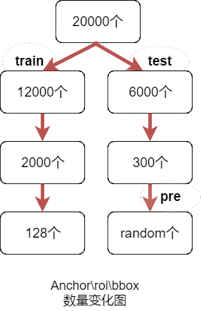
- 对于每张图片,利用它的特征图,计算$\frac{H}{16} \times \frac{W}{16} \times 9$(大约20000个)Anchor属于前景的概率以及对应的位置参数。
- 选取概率较大的12000个Anchor。
- 利用回归的位置参数修正这12000个Anchor的位置,获得ROIs。
- 利用非极大值抑制,选出概率最大的2000个ROIs。
注意! 在推理阶段,为了提高处理速度,12000和2000分别变成了6000和300。并且这部分操作不需要反向传播,所以可以利用numpy或者tensor实现。因此,RPN的输出就是形如$2000×4$或者$300×4$的Tensor。
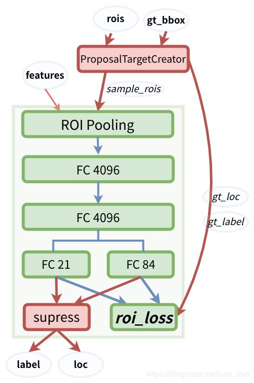
RPN给出了候选框,然后ROI Head就是在候选框的基础上继续进行分类和位置参数的回归获得最后的结果,ROI Head的结构图如下所示:
代码实现在model/utils/creator_tool.py里面,具体如下:
# 下面是ProposalCreator的代码: 这部分的操作不需要进行反向传播
# 因此可以利用numpy/tensor实现
class ProposalCreator:
    # 对于每张图片,利用它的feature map,计算(H/16)x(W/16)x9(大概20000)
    # 个anchor属于前景的概率,然后从中选取概率较大的12000张,利用位置回归参
    # 数,修正这12000个anchor的位置, 利用非极大值抑制,选出2000个ROIS以及
    # 对应的位置参数。
    def __init__(self,
                 parent_model,
                 nms_thresh=0.7,
                 n_train_pre_nms=12000,
                 n_train_post_nms=2000,
                 n_test_pre_nms=6000,
                 n_test_post_nms=300,
                 min_size=16
                 ):
        self.parent_model = parent_model
        self.nms_thresh = nms_thresh
        self.n_train_pre_nms = n_train_pre_nms
        self.n_train_post_nms = n_train_post_nms
        self.n_test_pre_nms = n_test_pre_nms
        self.n_test_post_nms = n_test_post_nms
        self.min_size = min_size
    # 这里的loc和score是经过region_proposal_network中
    # 经过1x1卷积分类和回归得到的。
    def __call__(self, loc, score,
                 anchor, img_size, scale=1.):

        if self.parent_model.training:
            n_pre_nms = self.n_train_pre_nms #12000
            n_post_nms = self.n_train_post_nms #经过NMS后有2000个
        else:
            n_pre_nms = self.n_test_pre_nms #6000
            n_post_nms = self.n_test_post_nms #经过NMS后有300个

        # 将bbox转换为近似groudtruth的anchor(即rois)
        roi = loc2bbox(anchor, loc)

        # slice表示切片操作
        # 裁剪将rois的ymin,ymax限定在[0,H]
        roi[:, slice(0, 4, 2)] = np.clip(
            roi[:, slice(0, 4, 2)], 0, img_size[0])
        # 裁剪将rois的xmin,xmax限定在[0,W]
        roi[:, slice(1, 4, 2)] = np.clip(
            roi[:, slice(1, 4, 2)], 0, img_size[1])

        # Remove predicted boxes with either height or width < threshold.
        min_size = self.min_size * scale #16
        # rois的宽
        hs = roi[:, 2] - roi[:, 0]
        # rois的高
        ws = roi[:, 3] - roi[:, 1]
        # 确保rois的长宽大于最小阈值
        keep = np.where((hs >= min_size) & (ws >= min_size))[0]
        roi = roi[keep, :]
        # 对剩下的ROIs进行打分(根据region_proposal_network中rois的预测前景概率)
        score = score[keep]

        # Sort all (proposal, score) pairs by score from highest to lowest.
        # Take top pre_nms_topN (e.g. 6000).
        # 将score拉伸并逆序(从高到低)排序
        order = score.ravel().argsort()[::-1]
        # train时从20000中取前12000个rois,test取前6000个
        if n_pre_nms > 0:
            order = order[:n_pre_nms]
        roi = roi[order, :]

        # Apply nms (e.g. threshold = 0.7).
        # Take after_nms_topN (e.g. 300).

        # unNOTE: somthing is wrong here!
        # TODO: remove cuda.to_gpu
        # #(具体需要看NMS的原理以及输入参数的作用)调用非极大值抑制函数,
        # 将重复的抑制掉,就可以将筛选后ROIS进行返回。经过NMS处理后Train
        # 数据集得到2000个框,Test数据集得到300个框
        keep = non_maximum_suppression(
            cp.ascontiguousarray(cp.asarray(roi)),
            thresh=self.nms_thresh)
        if n_post_nms > 0:
            keep = keep[:n_post_nms]
        # 取出最终的2000或300个rois
        roi = roi[keep]
        return roi
ProposalTargetCreator
ROIs给出了2000个候选框,分别对应了不同大小的Anchor。我们首先需要利用ProposalTargetCreator挑选出128个sample_rois,然后使用了ROI Pooling将这些不同尺寸的区域全部Pooling到同一个尺度($7×7$)上,关于ROI Pooling这里就不多讲了,具体见:实例分割算法之Mask R-CNN论文解读 。那么这里为什么要Pooling成$7×7$大小呢?
这是为了共享权重,前面在Extrator部分说到Faster RCNN除了前面基层卷积被用到之外,最后全连接层的权重也可以继续利用。当所有的RoIs都被Resize到$512×512×7$的特征图之后,将它Reshape成一个一维的向量,就可以利用VGG16预训练的权重初始化前两层全连接层了。最后,再接上两个全连接层FC21用来分类(20个类+背景,VOC)和回归(21个类,每个类有4个位置参数)。
我们再来看一下ProposalTargetCreator具体是如何选择128个ROIs进行训练的?过程如下:
- RoIs和GT box的IOU大于0.5的,选择一些如32个。
- RoIs和gt_bboxes的IoU小于等于0(或者0.1)的选择一些(比如 128-32=96个)作为负样本。
同时为了方便训练,对选择出的128个RoIs的gt_roi_loc进行标准化处理(减均值除以标准差)。
下面来看看代码实现,同样是在model/utils/creator_tool.py里面:
# 下面是ProposalTargetCreator代码:ProposalCreator产生2000个ROIS,
# 但是这些ROIS并不都用于训练,经过本ProposalTargetCreator的筛选产生
# 128个用于自身的训练

class ProposalTargetCreator(object):
    def __init__(self,
                 n_sample=128,
                 pos_ratio=0.25, pos_iou_thresh=0.5,
                 neg_iou_thresh_hi=0.5, neg_iou_thresh_lo=0.0
                 ):
        self.n_sample = n_sample
        self.pos_ratio = pos_ratio
        self.pos_iou_thresh = pos_iou_thresh
        self.neg_iou_thresh_hi = neg_iou_thresh_hi
        self.neg_iou_thresh_lo = neg_iou_thresh_lo  # NOTE:default 0.1 in py-faster-rcnn
    # 输入:2000个rois、一个batch(一张图)中所有的bbox ground truth(R,4)、
    # 对应bbox所包含的label(R,1)(VOC2007来说20类0-19)
    # 输出:128个sample roi(128,4)、128个gt_roi_loc(128,4)、
    # 128个gt_roi_label(128,1)
    def __call__(self, roi, bbox, label,
                 loc_normalize_mean=(0., 0., 0., 0.),
                 loc_normalize_std=(0.1, 0.1, 0.2, 0.2)):
        n_bbox, _ = bbox.shape
        # 首先将2000个roi和m个bbox给concatenate了一下成为
        # 新的roi(2000+m,4)。
        roi = np.concatenate((roi, bbox), axis=0)
        # n_sample = 128,pos_ratio=0.5,round 对传入的数据进行四舍五入
        pos_roi_per_image = np.round(self.n_sample * self.pos_ratio)
        # 计算每一个roi与每一个bbox的iou
        iou = bbox_iou(roi, bbox)
        # 按行找到最大值,返回最大值对应的序号以及其真正的IOU。
        # 返回的是每个roi与哪个bbox的最大,以及最大的iou值
        gt_assignment = iou.argmax(axis=1)
        # 每个roi与对应bbox最大的iou
        max_iou = iou.max(axis=1)
        # 从1开始的类别序号,给每个类得到真正的label(将0-19变为1-20)
        gt_roi_label = label[gt_assignment] + 1

        # 同样的根据iou的最大值将正负样本找出来,pos_iou_thresh=0.5
        pos_index = np.where(max_iou >= self.pos_iou_thresh)[0]
        # 需要保留的roi个数(满足大于pos_iou_thresh条件的roi与64之间较小的一个)
        pos_roi_per_this_image = int(min(pos_roi_per_image, pos_index.size))
        # 找出的样本数目过多就随机丢掉一些
        if pos_index.size > 0:
            pos_index = np.random.choice(
                pos_index, size=pos_roi_per_this_image, replace=False)

        # neg_iou_thresh_hi=0.5,neg_iou_thresh_lo=0.0
        neg_index = np.where((max_iou < self.neg_iou_thresh_hi) &
                             (max_iou >= self.neg_iou_thresh_lo))[0]
        neg_roi_per_this_image = self.n_sample - pos_roi_per_this_image
        neg_roi_per_this_image = int(min(neg_roi_per_this_image,
                                         neg_index.size))
        if neg_index.size > 0:
            neg_index = np.random.choice(
                neg_index, size=neg_roi_per_this_image, replace=False)

        # The indices that we're selecting (both positive and negative).
        keep_index = np.append(pos_index, neg_index)
        gt_roi_label = gt_roi_label[keep_index]
        gt_roi_label[pos_roi_per_this_image:] = 0  # 负样本label 设为0
        sample_roi = roi[keep_index]
        # 此时输出的128*4的sample_roi就可以去扔到 RoIHead网络里去进行分类
        # 与回归了。同样, RoIHead网络利用这sample_roi+featue为输入,输出
        # 是分类(21类)和回归(进一步微调bbox)的预测值,那么分类回归的groud
        # truth就是ProposalTargetCreator输出的gt_roi_label和gt_roi_loc。
        # Compute offsets and scales to match sampled RoIs to the GTs.
        # 求这128个样本的groundtruth
        gt_roi_loc = bbox2loc(sample_roi, bbox[gt_assignment[keep_index]])
        # ProposalTargetCreator首次用到了真实的21个类的label,
        # 且该类最后对loc进行了归一化处理,所以预测时要进行均值方差处理
        gt_roi_loc = ((gt_roi_loc - np.array(loc_normalize_mean, np.float32)
                       ) / np.array(loc_normalize_std, np.float32))

        return sample_roi, gt_roi_loc, gt_roi_label
📟 Faster RCNN网络模型搭建
注意网络结构图中的蓝色箭头的线代表了计算图,梯度反向传播会经过。而红色的线不需要反向传播。一个有趣的事情是在Instance-aware Semantic Segmentation via Multi-task Network Cascades这篇论文(https://arxiv.org/abs/1512.04412)中提到ProposalCreator生成RoIs的过程也可以进行反向传播,感兴趣可以去看看。
在上一节主要讲了RPN里面的AnchorTargetCreator,ProposalCreator,ProposalTargetCreator,而RPN网络的核心类RegionProposalNetwork还没讲,这里先看一下,代码在model/region_proposal_network.py里面,细节如下:
class RegionProposalNetwork(nn.Module):

    def __init__(
            self, in_channels=512, mid_channels=512, ratios=[0.5, 1, 2],
            anchor_scales=[8, 16, 32], feat_stride=16,
            proposal_creator_params=dict(),
    ):
        super(RegionProposalNetwork, self).__init__()
        # 首先生成上述以(0,0)为中心的9个base anchor
        self.anchor_base = generate_anchor_base(
            anchor_scales=anchor_scales, ratios=ratios)
        self.feat_stride = feat_stride
        self.proposal_layer = ProposalCreator(self, **proposal_creator_params)
        n_anchor = self.anchor_base.shape[0]
        self.conv1 = nn.Conv2d(in_channels, mid_channels, 3, 1, 1)
        self.score = nn.Conv2d(mid_channels, n_anchor * 2, 1, 1, 0)
        self.loc = nn.Conv2d(mid_channels, n_anchor * 4, 1, 1, 0)
        normal_init(self.conv1, 0, 0.01)
        normal_init(self.score, 0, 0.01)
        normal_init(self.loc, 0, 0.01)

    def forward(self, x, img_size, scale=1.):
       # x的尺寸为(batch_size,512,H/16,W/16),其中H,W分别为原图的高和宽
        # x为feature map,n为batch_size,此版本代码为1. hh,ww即为宽高
        n, _, hh, ww = x.shape
        # 在9个base_anchor基础上生成hh*ww*9个anchor,对应到原图坐标
        # feat_stride=16 ,因为是经4次pool后提到的特征,故feature map较
        # 原图缩小了16倍
        anchor = _enumerate_shifted_anchor(
            np.array(self.anchor_base),/
            self.feat_stride, hh, ww)

        # (hh * ww * 9)/hh*ww = 9
        n_anchor = anchor.shape[0] // (hh * ww)
        # 512个3x3卷积(512, H/16,W/16)
        h = F.relu(self.conv1(x))
        # n_anchor(9)* 4个1x1卷积,回归坐标偏移量。(9*4,hh,ww)
        rpn_locs = self.loc(h)
        # UNNOTE: check whether need contiguous
        # A: Yes
        # 转换为(n,hh,ww,9*4)后变为(n,hh*ww*9,4)
        rpn_locs = rpn_locs.permute(0, 2, 3, 1).contiguous().view(n, -1, 4)
        # n_anchor(9)*2个1x1卷积,回归类别。(9*2,hh,ww)
        rpn_scores = self.score(h)
        # 转换为(n,hh,ww,9*2)
        rpn_scores = rpn_scores.permute(0, 2, 3, 1).contiguous()
        # 计算{Softmax}(x_{i}) = \{enp(x_i)}{\sum_j enp(x_j)}
        rpn_softmax_scores = F.softmax(rpn_scores.view(n, hh, ww, n_anchor, 2), dim=4)
        # 得到前景的分类概率
        rpn_fg_scores = rpn_softmax_scores[:, :, :, :, 1].contiguous()
        # 得到所有anchor的前景分类概率
        rpn_fg_scores = rpn_fg_scores.view(n, -1)
        # 得到每一张feature map上所有anchor的网络输出值
        rpn_scores = rpn_scores.view(n, -1, 2)

        rois = list()
        roi_indices = list()
        # n为batch_size数
        for i in range(n):
            # 调用ProposalCreator函数, rpn_locs维度(hh*ww*9,4)
            # ,rpn_fg_scores维度为(hh*ww*9),anchor的维度为
            # (hh*ww*9,4), img_size的维度为(3,H,W),H和W是
            # 经过数据预处理后的。计算(H/16)x(W/16)x9(大概20000)
            # 个anchor属于前景的概率,取前12000个并经过NMS得到2000个
            # 近似目标框G^的坐标。roi的维度为(2000,4)
            roi = self.proposal_layer(
                rpn_locs[i].cpu().data.numpy(),
                rpn_fg_scores[i].cpu().data.numpy(),
                anchor, img_size,
                scale=scale)
            batch_index = i * np.ones((len(roi),), dtype=np.int32)
            # rois为所有batch_size的roi
            rois.append(roi)
            roi_indices.append(batch_index)
        # 按行拼接(即没有batch_size的区分,每一个[]里都是一个anchor的四个坐标)
        rois = np.concatenate(rois, axis=0)
        # 这个 roi_indices在此代码中是多余的,因为我们实现的是batch_siae=1的
        # 网络,一个batch只会输入一张图象。如果多张图像的话就需要存储索引以找到
        # 对应图像的roi
        roi_indices = np.concatenate(roi_indices, axis=0)
        # rpn_locs的维度(hh*ww*9,4),rpn_scores维度为(hh*ww*9,2),
        # rois的维度为(2000,4),roi_indices用不到,
        # anchor的维度为(hh*ww*9,4)
        return rpn_locs, rpn_scores, rois, roi_indices, anchor
可以看到RegionProposalNetwork继承于nn.Module,这个网络我们在上一个推文讲的很细节了,在继续阅读之前,请确保你已经理解了RPN和ROI Head。
接下来,我们需要知道在model/roi_module.py里面主要利用了cupy(专用于GPU的numpy)实现ROI Pooling的前向传播和反向传播。NMS和ROI pooling利用了:「cupy」和「chainer」 。
其主要任务是对于一张图像得到的特征图(),然后利用sample_roi的bbox坐标去在特征图上裁剪下来所有roi对应的特征图(训练:)、(测试:)。
接下来就是搭建网络模型的文件model/faster_rcnn.py,这个脚本定义了Faster RCNN的基本类「FasterRCNN」。我们知道Faster RCNN的三个核心步骤就是:
- 特征提取:输入一张图片得到其特征图feature map
- RPN:给定特征图后产生一系列RoIs
- ROI Head:利用这些RoIs对应的特征图对这些RoIs中的类别进行分类,并提升定位精度
在「FasterRCNN」这个类中就初始化了这三个重要的步骤,即self.extrator,self.rpn,self.head。
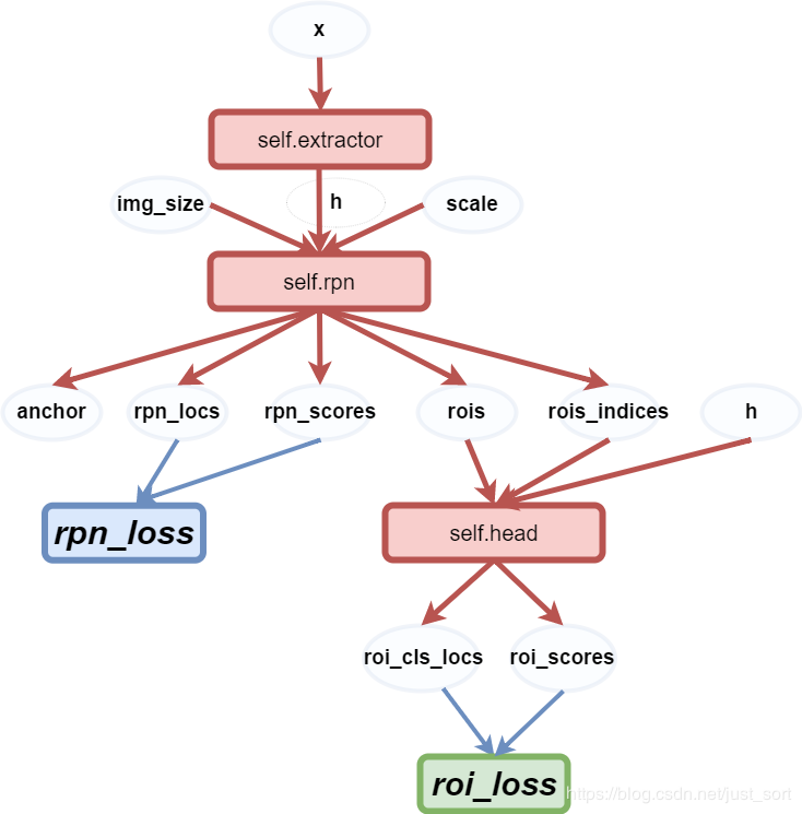
「FasterRCNN」类中,forward函数实现前向传播,代码如下:
def forward(self, x, scale=1.):
        # 实现前向传播
        img_size = x.shape[2:]

        h = self.extractor(x)
        rpn_locs, rpn_scores, rois, roi_indices, anchor = \
            self.rpn(h, img_size, scale)
        roi_cls_locs, roi_scores = self.head(
            h, rois, roi_indices)
        return roi_cls_locs, roi_scores, rois, roi_indices
也可以用下图来更清晰的表示:
而这个forward过程中边界框的数量变化可以表示为下图:
接下来我们看一下预测函数predict,这个函数实现了对测试集图片的预测,同样batch=1,即每次输入一张图片。详解如下:
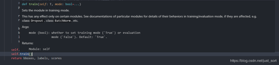
def predict(self, imgs,sizes=None,visualize=False):
        # 设置为eval模式
        self.eval()
        # 是否开启可视化
        if visualize:
            self.use_preset('visualize')
            prepared_imgs = list()
            sizes = list()
            for img in imgs:
                size = img.shape[1:]
                img = preprocess(at.tonumpy(img))
                prepared_imgs.append(img)
                sizes.append(size)
        else:
             prepared_imgs = imgs
        bboxes = list()
        labels = list()
        scores = list()
        for img, size in zip(prepared_imgs, sizes):
            img = at.totensor(img[None]).float()
            # 对读入的图片求尺度scale,因为输入的图像经预处理就会有缩放,
            # 所以需记录缩放因子scale,这个缩放因子在ProposalCreator
            # 筛选roi时有用到,即将所有候选框按这个缩放因子映射回原图,
            # 超出原图边框的趋于将被截断。
            scale = img.shape[3] / size[1]
            # 执行forward
            roi_cls_loc, roi_scores, rois, _ = self(img, scale=scale)
            # We are assuming that batch size is 1.

            roi_score = roi_scores.data
            roi_cls_loc = roi_cls_loc.data
            roi = at.totensor(rois) / scale

            # Convert predictions to bounding boxes in image coordinates.
            # Bounding boxes are scaled to the scale of the input images.
            # 为ProposalCreator对loc做了归一化(-mean /std)处理,所以这里
            # 需要再*std+mean,此时的位置参数loc为roi_cls_loc。然后将这128
            # 个roi利用roi_cls_loc进行微调,得到新的cls_bbox。
            mean = t.Tensor(self.loc_normalize_mean).cuda(). \
                repeat(self.n_class)[None]
            std = t.Tensor(self.loc_normalize_std).cuda(). \
                repeat(self.n_class)[None]

            roi_cls_loc = (roi_cls_loc * std + mean)
            roi_cls_loc = roi_cls_loc.view(-1, self.n_class, 4)
            roi = roi.view(-1, 1, 4).enpand_as(roi_cls_loc)
            cls_bbox = loc2bbox(at.tonumpy(roi).reshape((-1, 4)),
                                at.tonumpy(roi_cls_loc).reshape((-1, 4)))
            cls_bbox = at.totensor(cls_bbox)
            cls_bbox = cls_bbox.view(-1, self.n_class * 4)
            # clip bounding box
            cls_bbox[:, 0::2] = (cls_bbox[:, 0::2]).clamp(min=0, max=size[0])
            cls_bbox[:, 1::2] = (cls_bbox[:, 1::2]).clamp(min=0, max=size[1])
            # 对于分类得分roi_scores,我们需要将其经过softmax后转为概率prob。
            # 值得注意的是我们此时得到的是对所有输入128个roi以及位置参数、得分
            # 的预处理,下面将筛选出最后最终的预测结果。
            prob = at.tonumpy(F.softmax(at.totensor(roi_score), dim=1))

            raw_cls_bbox = at.tonumpy(cls_bbox)
            raw_prob = at.tonumpy(prob)

            bbox, label, score = self._suppress(raw_cls_bbox, raw_prob)
            bboxes.append(bbox)
            labels.append(label)
            scores.append(score)

        self.use_preset('evaluate')
        self.train()
        return bboxes, labels, scores
「注意!」 训练完train_datasets之后,model要来测试样本了。在model(test_datasets)之前,需要加上model.eval()。否则的话,有输入数据,即使不训练,它也会改变权值。这是model中含有batch normalization层所带来的的性质。
所以我们看到在第一行使用了self.eval(),那么为什么在最后一行函数返回bboxes,labels,scores之后还要加一行self.train呢?这是因为这次预测之后下次要接着训练,训练的时候需要设置模型类型为train。
上面的步骤是对网络RoIhead网络输出的预处理,函数_suppress将得到真正的预测结果。_suppress函数解释如下:
# predict函数是对网络RoIhead网络输出的预处理
    # 函数_suppress将得到真正的预测结果。
    # 此函数是一个按类别的循环,l从1至20(0类为背景类)。
    # 即预测思想是按20个类别顺序依次验证,如果有满足该类的预测结果,
    # 则记录,否则转入下一类(一张图中也就几个类别而已)。例如筛选
    # 预测出第1类的结果,首先在cls_bbox中将所有128个预测第1类的
    # bbox坐标找出,然后从prob中找出128个第1类的概率。因为阈值为0.7,
    # 也即概率>0.7的所有边框初步被判定预测正确,记录下来。然而可能有
    # 多个边框预测第1类中同一个物体,同类中一个物体只需一个边框,
    # 所以需再经基于类的NMS后使得每类每个物体只有一个边框,至此
    # 第1类预测完成,记录第1类的所有边框坐标、标签、置信度。
    # 接着下一类...,直至20类都记录下来,那么一张图片(也即一个batch)
    # 的预测也就结束了。
    def _suppress(self, raw_cls_bbox, raw_prob):
        bbox = list()
        label = list()
        score = list()
        # skip cls_id = 0 because it is the background class
        for l in range(1, self.n_class):
            cls_bbox_l = raw_cls_bbox.reshape((-1, self.n_class, 4))[:, l, :]
            prob_l = raw_prob[:, l]
            mask = prob_l > self.score_thresh
            cls_bbox_l = cls_bbox_l[mask]
            prob_l = prob_l[mask]
            keep = non_maximum_suppression(
                cp.array(cls_bbox_l), self.nms_thresh, prob_l)
            keep = cp.asnumpy(keep)
            bbox.append(cls_bbox_l[keep])
            # The labels are in [0, self.n_class - 2].
            label.append((l - 1) * np.ones((len(keep),)))
            score.append(prob_l[keep])
        bbox = np.concatenate(bbox, axis=0).astype(np.float32)
        label = np.concatenate(label, axis=0).astype(np.int32)
        score = np.concatenate(score, axis=0).astype(np.float32)
        return bbox, label, score
这里还定义了优化器optimizer,对于需要求导的参数 按照是否含bias赋予不同的学习率。默认是使用SGD,可选Adam,不过需更小的学习率。代码如下:
# 定义了优化器optimizer,对于需要求导的参数 按照是否含bias赋予不同的学习率。
    # 默认是使用SGD,可选Adam,不过需更小的学习率。
    def get_optimizer(self):
        """
        return optimizer, It could be overwriten if you want to specify
        special optimizer
        """
        lr = opt.lr
        params = []
        for key, value in dict(self.named_parameters()).items():
            if value.requires_grad:
                if 'bias' in key:
                    params += [{'params': [value], 'lr': lr * 2, 'weight_decay': 0}]
                else:
                    params += [{'params': [value], 'lr': lr, 'weight_decay': opt.weight_decay}]
        if opt.use_adam:
            self.optimizer = t.optim.Adam(params)
        else:
            self.optimizer = t.optim.SGD(params, momentum=0.9)
        return self.optimizer

    def scale_lr(self, decay=0.1):
        for param_group in self.optimizer.param_groups:
            param_group['lr'] *= decay
        return self.optimizer
解释完了这个基类,我们来看看这份代码里面实现的基于VGG16的Faster RCNN的这个类FasterRCNNVGG16,它继承了「FasterRCNN」。
首先引入VGG16,然后拆分为特征提取网络和分类网络。冻结分类网络的前几层,不进行反向传播。
然后实现「VGG16RoIHead」网络。实现输入特征图、rois、roi_indices,输出roi_cls_locs和roi_scores。
类FasterRCNNVGG16分别对VGG16的特征提取部分、分类部分、RPN网络、VGG16RoIHead网络进行了实例化。
此外在对VGG16RoIHead网络的全连接层权重初始化过程中,按照图像是否为truncated(截断)分了两种初始化分方法,至于这个截断具体有什么用呢,也不是很明白这里似乎也没用。
详细解释如下:
def decom_vgg16():
    # the 30th layer of features is relu of conv5_3
    # 是否使用Caffe下载下来的预训练模型
    if opt.caffe_pretrain:
        model = vgg16(pretrained=False)
        if not opt.load_path:
            # 加载参数信息
            model.load_state_dict(t.load(opt.caffe_pretrain_path))
    else:
        model = vgg16(not opt.load_path)

    # 加载预训练模型vgg16的conv5_3之前的部分
    features = list(model.features)[:30]

    classifier = model.classifier
    # 分类部分放到一个list里面
    classifier = list(classifier)
    # 删除输出分类结果层
    del classifier[6]
    # 删除两个dropout
    if not opt.use_drop:
        del classifier[5]
        del classifier[2]
    classifier = nn.Sequential(*classifier)

    # 冻结vgg16前2个stage,不进行反向传播
    for layer in features[:10]:
        for p in layer.parameters():
            p.requires_grad = False
    # 拆分为特征提取网络和分类网络
    return nn.Sequential(*features), classifier


# 分别对特征VGG16的特征提取部分、分类部分、RPN网络、
# VGG16RoIHead网络进行了实例化
class FasterRCNNVGG16(FasterRCNN):
    # vgg16通过5个stage下采样16倍
    feat_stride = 16  # downsample 16x for output of conv5 in vgg16
    # 总类别数为20类,三种尺度三种比例的anchor
    def __init__(self,
                 n_fg_class=20,
                 ratios=[0.5, 1, 2],
                 anchor_scales=[8, 16, 32]
                 ):

        # conv5_3及之前的部分,分类器
        extractor, classifier = decom_vgg16()

        # 返回rpn_locs, rpn_scores, rois, roi_indices, anchor
        rpn = RegionProposalNetwork(
            512, 512,
            ratios=ratios,
            anchor_scales=anchor_scales,
            feat_stride=self.feat_stride,
        )
        # 下面讲
        head = VGG16RoIHead(
            n_class=n_fg_class + 1,
            roi_size=7,
            spatial_scale=(1. / self.feat_stride),
            classifier=classifier
        )

        super(FasterRCNNVGG16, self).__init__(
            extractor,
            rpn,
            head,
        )


class VGG16RoIHead(nn.Module):
    def __init__(self, n_class, roi_size, spatial_scale,
                 classifier):
        # n_class includes the background
        super(VGG16RoIHead, self).__init__()
        # vgg16中的最后两个全连接层
        self.classifier = classifier
        self.cls_loc = nn.Linear(4096, n_class * 4)
        self.score = nn.Linear(4096, n_class)
        # 全连接层权重初始化
        normal_init(self.cls_loc, 0, 0.001)
        normal_init(self.score, 0, 0.01)
        # 加上背景21类
        self.n_class = n_class
        # 7x7
        self.roi_size = roi_size
        # 1/16
        self.spatial_scale = spatial_scale
        # 将大小不同的roi变成大小一致,得到pooling后的特征,
        # 大小为[300, 512, 7, 7]。利用Cupy实现在线编译的
        self.roi = RoIPooling2D(self.roi_size, self.roi_size, self.spatial_scale)

    def forward(self, x, rois, roi_indices):
        # 前面解释过这里的roi_indices其实是多余的,因为batch_size一直为1
        # in case roi_indices is  ndarray
        roi_indices = at.totensor(roi_indices).float() #ndarray->tensor
        rois = at.totensor(rois).float()
        indices_and_rois = t.cat([roi_indices[:, None], rois], dim=1)
        # NOTE: important: yx->xy
        xy_indices_and_rois = indices_and_rois[:, [0, 2, 1, 4, 3]]
        # 把tensor变成在内存中连续分布的形式
        indices_and_rois =  xy_indices_and_rois.contiguous()
        # 接下来分析roi_module.py中的RoI()
        pool = self.roi(x, indices_and_rois)
        # flat操作
        pool = pool.view(pool.size(0), -1)
        # decom_vgg16()得到的calssifier,得到4096
        fc7 = self.classifier(pool)
        # (4096->84)
        roi_cls_locs = self.cls_loc(fc7)
        # (4096->21)
        roi_scores = self.score(fc7)
        return roi_cls_locs, roi_scores


def normal_init(m, mean, stddev, truncated=False):
    """
    weight initalizer: truncated normal and random normal.
    """
    # x is a parameter
    if truncated:
        m.weight.data.normal_().fmod_(2).mul_(stddev).add_(mean)  # not a perfect approximation
    else:
        m.weight.data.normal_(mean, stddev)
m.bias.data.zero_()本博客所有文章除特别声明外,均采用 CC BY-SA 4.0 协议 ,转载请注明出处!